What is gorder?

gorder is a command-line tool that aims to provide a comprehensive, reliable, simple, and fast way to calculate atomistic and coarse-grained lipid order parameters from Gromacs simulations.

The primary (and possibly naïve) goal of gorder is to completely replace the use of gmx order for atomistic and coarse-grained systems. gmx order is a tool still widely used in the Gromacs community despite its tedious usage and the fact that it sometimes produces completely incorrect results.¹

Apart from calculating the order parameters correctly, gorder also offers many additional features, such as reporting order parameters for individual C-H bonds, error estimation, leaflet classification, geometric selection, or construction of ordermaps. gorder can also calculate order parameters for non-planar membranes such as tubes or vesicles.

gorder is written in Rust and is also available as a Rust crate. If you want to see the code (or comparison with other programs), visit the gorder GitHub repository.

Even Gromacs developers say that you should not use gmx order.

Some theory

Lipid order parameters quantify the degree of ordering in lipid membranes. They can be obtained from both experimental measurements and simulations, making them quite useful for checking force-field accuracy, studying molecular structures, tracking phase transitions and various other stuff.

The order parameter $S$ in atomistic simulations can be calculated as:

$S = \frac{1}{2} ⟨ 3 cos^{2} θ - 1 ⟩$

where $θ$ is the angle between the C-H bond vector and the bilayer normal, and the angular brackets represent molecular and temporal ensemble averages. The order parameter for atomistic systems is usually reported as the negative of this calculated value, $- S$ (often denoted as $- S_{C H}$ or $- S_{C D}$ ). Higher positive values of $- S$ indicate more ordered membrane structures.

For coarse-grained systems, the order parameter can be calculated using the same equation. However, here $θ$ corresponds to the angle between the vector connecting two consecutive beads of the lipid and the bilayer normal. Using this definition, the order parameter $S$ (sometimes denoted as $S_{CC}$ ) increases as the membrane structure becomes more ordered. For coarse-grained systems, the order parameter is usually reported directly as $S$ to facilitate comparison with the atomistic $- S$ (which follows the same trend).

Installation

Installing the gorder tool consists of two simple steps:

Install Rust.
- Follow this guide for your operating system.
- If you already have Rust installed, you can skip this step. To check, run rustc --version.
You need Rust v1.82 or newer to be able to install gorder. To update Rust, run rustup update.
Install gorder.
- Run cargo install gorder in your terminal.

You can verify that the installation was successful by running gorder --version. The current version of the gorder tool should be displayed in the terminal. If everything went right, you can now call gorder from anywhere.

Atomistic order parameters

Preparing the input

Suppose we have a CHARMM36 membrane composed of POPC, POPE, and POPG lipids.

To calculate atomistic order parameters, we need two Gromacs files:

A TPR file containing the system structure and topology (system.tpr).
An XTC trajectory file (md.xtc) whose frames will be analyzed.

It is recommended to use TPR and XTC files, but gorder also supports various other file formats.

Next, we create an input YAML file that specifies the options for the analysis:

structure: system.tpr
trajectory: md.xtc
analysis_type: !AAOrder
  heavy_atoms: "@membrane and name r'C3.+|C2.+'"
  hydrogens: "@membrane and element name hydrogen"
output: order.yaml

In the input YAML file, the analysis type AAOrder requires you to specify both heavy_atoms and hydrogens. gorder will then identify all bonds connecting the selected heavy atoms with the selected hydrogen atoms. The order parameters are calculated for all these identified bonds.

The atoms are selected using a query language called GSL. If you are familiar with the query language used in VMD, you'll find the basic syntax of GSL intuitive.

Here:

heavy_atoms are selected using the query @membrane and name r'C3.+|C2.+', which selects all palmitoyl and oleoyl carbons of the membrane lipids.
hydrogens are selected using the query @membrane and element name hydrogen.

@membrane is a GSL autodetection macro that selects all atoms of common membrane lipids. r'C3.+|C2.+' is a regular expression block, natively supported by GSL.

The results of the analysis will be saved in the order.yaml file as $- S_{C H}$ (see Theory).

Running the analysis

We save the input YAML file, for example, as analyze.yaml. Then, we run gorder as follows:

$ gorder analyze.yaml

During the analysis, we will see something like this:

Note that the structure from the TPR file is not analyzed. The TPR file is only used to construct the system and obtain its topology.

The results of the analysis are saved in the order.yaml file. Here is an excerpt from the file:

# Order parameters calculated with 'gorder v0.5.0' using structure file 'system.tpr' and trajectory file 'md.xtc'.
average order:
  total: 0.1631
POPE:
  average order:
    total: 0.1601
  order parameters:
    POPE C22 (23):
      total: 0.1036
      bonds:
        POPE H2R (24):
          total: 0.0876
        POPE H2S (25):
          total: 0.1196
    POPE C32 (32):
      total: 0.2297
      bonds:
        POPE H2X (33):
          total: 0.2423
        POPE H2Y (34):
          total: 0.2171
  # (...)
POPC:
  average order:
    total: 0.166
  order parameters:
    POPC C22 (32):
      total: 0.1109
      bonds:
        POPC H2R (33):
          total: 0.0935
        POPC H2S (34):
          total: 0.1283
    POPC C32 (41):
      total: 0.2373
      bonds:
        POPC H2X (42):
          total: 0.2483
        POPC H2Y (43):
          total: 0.2264
  # (...)
POPG:
  average order:
    total: 0.1608
  order parameters:
    POPG C22 (25):
      total: 0.0987
      bonds:
        POPG H2R (26):
          total: 0.08
        POPG H2S (27):
          total: 0.1174
    POPG C32 (34):
      total: 0.2272
      bonds:
        POPG H2X (35):
          total: 0.2367
        POPG H2Y (36):
          total: 0.2177

gorder automatically identified three molecule types and all relevant bonds. Order parameters are reported separately for each molecule type: for each bond type of each molecule type and for each heavy atom type of each molecule type. Order parameters for heavy atom types are obtained by averaging the order parameters of their bonds with hydrogens. average order corresponds to the average order of all the relevant bonds of the entire system or a single molecule type, respectively.

The atom types (and molecule types) are listed in the same order as they appear in the input TPR structure. Note that parameters for C21 and C31 are absent, even though these atoms should qualify as heavy_atoms based on the regular expression C3.+|C2.+. However, these atoms lack bonded hydrogens and are therefore automatically excluded from the output.

Let's take a closer look at a part of the YAML file:

average order:
  total: 0.1631          # average order calculated for all molecules in the entire membrane
POPE:                    # name of the molecule
  average_order:
    total: 0.1601        # average order calculated for POPE molecules in the entire membrane
  order parameters:
    POPC C22 (23):       # heavy atom type: residue atom_name (relative_index)
      total: 0.1036      # order parameter of the heavy atom
      bonds:             # bonds of this heavy atom with hydrogens
        POPC H2R (24):   # hydrogen type: residue atom_name (relative_index)
          total: 0.0876  # order parameter of bond with this hydrogen
        POPC H2S (25):   # hydrogen type: residue atom_name (relative_index)
          total: 0.1196  # order parameter of bond with this hydrogen

YAML files are easy to read programmatically and not completely human-unreadable. However, gorder also provides other output formats (XVG, CSV, human-readable table). See Output formats for more information.

Using groups from an NDX file

gorder also supports using groups from NDX files. Let's suppose our NDX file already contains a group called TailCarbons, which specifies all the carbons to use. We no longer need to specify them using the complex regular expression from the previous example and can simply select the group. Our input YAML file will look like this:

structure: system.tpr
trajectory: md.xtc
index: index.ndx               # name of the NDX file
analysis_type: !AAOrder
  heavy_atoms: "TailCarbons"   # name of a group from NDX file
  hydrogens: "@membrane and element name hydrogen"
output: order.yaml

Then, we run the analysis in the same way as before.

Coarse-grained order parameters

Preparing the input

Suppose we have a Martini 3 membrane composed of POPC, POPE, and POPG lipids.

To calculate coarse-grained order parameters, we need two Gromacs files:

A TPR file containing the system structure and topology (system.tpr).
An XTC trajectory file (md.xtc) whose frames will be analyzed.

It is recommended to use TPR and XTC files, but gorder also supports various other file formats.

Next, we create an input YAML file that specifies the options for the analysis:

structure: system.tpr
trajectory: md.xtc
analysis_type: !CGOrder
  beads: "@membrane"
output: order.yaml

In the input YAML file, the analysis type CGOrder requires you to specify beads that will be considered for the analysis. gorder will then identify all bonds connecting the selected beads. The order parameters are calculated for all these identified bonds.

The atoms are selected using a query language called GSL. If you are familiar with the query language used in VMD, you'll find the basic syntax of GSL intuitive.

Here beads are selected using the query @membrane. That is a GSL autodetection macro that select all beads or atoms of common membrane lipids.

The results of the analysis will be saved in the order.yaml file as $S$ (see Theory).

Running the analysis

We save the input YAML file, for example, as analyze.yaml. Then, we run gorder as follows:

$ gorder analyze.yaml

During the analysis, we will see something like this:

Note that the structure from the TPR file is not analyzed. The TPR file is only used to construct the system and obtain its topology.

The results of the analysis are saved in the order.yaml file. Here is an excerpt from the file:

# Order parameters calculated with 'gorder v0.5.0' using structure file 'system.tpr' and trajectory file 'md.xtc'.
average order:
  total: 0.2937
POPC:
  average order:
    total: 0.2902
  order parameters:
    POPC NC3 (0) - POPC PO4 (1):
      total: -0.1362
    POPC PO4 (1) - POPC GL1 (2):
      total: 0.585
    POPC GL1 (2) - POPC GL2 (3):
      total: -0.1808
    POPC GL1 (2) - POPC C1A (4):
      total: 0.3835
  # (...)
POPE:
  average order:
    total: 0.2959
  order parameters:
    POPE NH3 (0) - POPE PO4 (1):
      total: -0.1293
    POPE PO4 (1) - POPE GL1 (2):
      total: 0.6072
    POPE GL1 (2) - POPE GL2 (3):
      total: -0.1833
    POPE GL1 (2) - POPE C1A (4):
      total: 0.3965
  # (...)
POPG:
  average order:
    total: 0.3063
  order parameters:
    POPG GL0 (0) - POPG PO4 (1):
      total: 0.0004
    POPG PO4 (1) - POPG GL1 (2):
      total: 0.5917
    POPG GL1 (2) - POPG GL2 (3):
      total: -0.1807
    POPG GL1 (2) - POPG C1A (4):
      total: 0.395
  # (...)

gorder automatically identified three molecule types and all relevant bonds. Order parameters are reported for each bond type of each molecule type. average order corresponds to the average order of all the relevant bonds of the entire system or a single molecule type, respectively.

The bond types (and molecule types) are listed in the same order their atoms appear in the input TPR structure.

Let's take a closer look at a part of the YAML file:

average order:
  total: 0.2937                   # average order calculated for all molecules in the entire membrane
POPC:                             # name of the molecule
  average order:
    total: 0.2902                 # average order calculated for POPC molecules in the entire membrane
  order parameters:
    POPC NC3 (0) - POPC PO4 (1):  # bond type (atom type 1 - atom type 2)
      total: -0.1362              # order parameter of this bond
    POPC PO4 (1) - POPC GL1 (2):  # atom types are specified as residue atom_name (relative_index)
      total: 0.585
    POPC GL1 (2) - POPC GL2 (3):
      total: -0.1808
    POPC GL1 (2) - POPC C1A (4):
      total: 0.3835

Using groups from an NDX file

gorder also supports using groups from NDX files. Let's suppose our NDX file already contains a group called LipidBeads, which specifies all the beads to use. We can then simply select the group. Our input YAML file will look like this:

structure: system.tpr
trajectory: md.xtc
index: index.ndx        # name of the NDX file
analysis_type: !CGOrder
  beads: "LipidBeads"   # name of a group from NDX file
output: order.yaml

Then, we run the analysis in the same way as before.

Output formats

The YAML output is always generated by gorder, as it contains all the calculated information. See Atomistic order parameters or Coarse-grained order parameters for more details about this format. However, gorder can also write output in other formats.

CSV format

CSV format may be useful if you want to work with the results using spreadsheet software such as LibreOffice Calc or Microsoft Excel, or when working with data analysis libraries like Pandas or Polars.

To write the results of the analysis in CSV format, add output_csv: PATH_TO_OUTPUT to your input YAML file.

Here is an excerpt from a CSV file:

molecule,residue,atom,relative index,total,hydrogen #1,hydrogen #2,hydrogen #3
POPE,POPE,C22,23,0.1036,0.0876,0.1196,
POPE,POPE,C32,32,0.2297,0.2423,0.2171,
POPE,POPE,C23,35,0.2138,0.2139,0.2138,
POPE,POPE,C24,38,0.2165,0.2158,0.2172,
POPE,POPE,C25,41,0.2290,0.2305,0.2274,
POPE,POPE,C26,44,0.2081,0.2099,0.2063,
POPE,POPE,C27,47,0.1989,0.2001,0.1977,
POPE,POPE,C28,50,0.1176,0.1163,0.1190,
POPE,POPE,C29,53,0.0703,0.0703,,
POPE,POPE,C210,55,0.0598,0.0598,,
(...)
POPE,POPE,C218,78,0.0321,0.0316,0.0327,0.0319
(...)
POPC,POPC,C22,32,0.1109,0.0935,0.1283,
POPC,POPC,C32,41,0.2373,0.2483,0.2264,
POPC,POPC,C23,44,0.2244,0.2237,0.2252,
POPC,POPC,C24,47,0.2230,0.2223,0.2236,
POPC,POPC,C25,50,0.2355,0.2358,0.2352,
POPC,POPC,C26,53,0.2122,0.2134,0.2109,
POPC,POPC,C27,56,0.2031,0.2035,0.2027,
POPC,POPC,C28,59,0.1196,0.1193,0.1199,
POPC,POPC,C29,62,0.0711,0.0711,,
POPC,POPC,C210,64,0.0610,0.0610,,
(...)
POPC,POPC,C218,87,0.0344,0.0340,0.0351,0.0340
(...)
POPG,POPG,C22,25,0.0987,0.0800,0.1174,
POPG,POPG,C32,34,0.2272,0.2367,0.2177,
POPG,POPG,C23,37,0.2088,0.2075,0.2101,
POPG,POPG,C24,40,0.2117,0.2108,0.2126,
POPG,POPG,C25,43,0.2254,0.2255,0.2253,
POPG,POPG,C26,46,0.2039,0.2006,0.2072,
POPG,POPG,C27,49,0.1933,0.1911,0.1954,
POPG,POPG,C28,52,0.1132,0.1148,0.1117,
POPG,POPG,C29,55,0.0637,0.0637,,
POPG,POPG,C210,57,0.0624,0.0624,,
(...)
POPG,POPG,C218,80,0.0330,0.0296,0.0324,0.0369

Each line corresponds to one heavy atom type (or one bond type in the case of coarse-grained systems). The first column corresponds to the molecule name, the second to the residue name, the third to the atom name, the fourth to the relative index of the atom type, the fifth to the order parameter calculated for this atom type, and the following columns correspond to the order parameters of the bonds the heavy atom type is involved in.

Table format

The Table format presents the results of the analysis in a clear, human-readable format.

To write the results of the analysis in Table format, add output_tab: PATH_TO_OUTPUT to your input YAML file.

Here is an excerpt from a Table file:

# Order parameters calculated with 'gorder v0.5.0' using structure file 'system.tpr' and trajectory file 'md.xtc'.

Molecule type POPE
           TOTAL   |   H #1   |   H #2   |   H #3   |
C22        0.1036  |  0.0876  |  0.1196  |          |
C32        0.2297  |  0.2423  |  0.2171  |          |
C23        0.2138  |  0.2139  |  0.2138  |          |
C24        0.2165  |  0.2158  |  0.2172  |          |
(...)
AVERAGE    0.1601  |

Molecule type POPC
           TOTAL   |   H #1   |   H #2   |   H #3   |
C22        0.1109  |  0.0935  |  0.1283  |          |
C32        0.2373  |  0.2483  |  0.2264  |          |
C23        0.2244  |  0.2237  |  0.2252  |          |
C24        0.2230  |  0.2223  |  0.2236  |          |
(...)
AVERAGE    0.1660  |

Molecule type POPG
           TOTAL   |   H #1   |   H #2   |   H #3   |
C22        0.0987  |  0.0800  |  0.1174  |          |
C32        0.2272  |  0.2367  |  0.2177  |          |
C23        0.2088  |  0.2075  |  0.2101  |          |
C24        0.2117  |  0.2108  |  0.2126  |          |
(...)
AVERAGE    0.1608  |

All molecule types
           TOTAL   |
AVERAGE    0.1631  |

Each line corresponds to one heavy atom type (or one bond type in the case of coarse-grained systems). The first column corresponds to the name of the atom type, the second to the order parameter calculated for this atom type, and the following columns correspond to the order parameters of the bond the heavy atom type is involved in. The last line in each molecule type (AVERAGE) corresponds to the average order of all the relevant bonds of a single molecule type. The last segment (All molecule types) shows average order parameter calculated for the entire system (all the identified molecules).

XVG format

XVG format may be useful if you want to quickly visualize the results as plots using xmgrace.

To write the results of the analysis in XVG format, add output_xvg: FILE_PATTERN to your input YAML file. One XVG file will be created for each molecule. The name of the molecule will be appended to the end of the file stem. For example, if your file pattern is order.xvg and the membrane contains POPC, POPE, and POPG lipid molecules, three XVG files will be generated: order_POPC.xvg, order_POPE.xvg, and order_POPG.xvg.

Here is an excerpt from an XVG file:

# Order parameters calculated with 'gorder v0.5.0' using structure file 'system.tpr' and trajectory file 'md.xtc'.
@    title "Atomistic order parameters for molecule type POPC"
@    xaxis label "Atom"
@    yaxis label "-Sch"
@    s0 legend "Full membrane"
@TYPE xy
# Atom C22:
1      0.1109
# Atom C32:
2      0.2373
# Atom C23:
3      0.2244
# Atom C24:
4      0.2230
# Atom C25:
5      0.2355
# Atom C26:
6      0.2122
# Atom C27:
7      0.2031
# Atom C28:
8      0.1196
(...)

XVG files provide the least complete information. The first column is the index of the analyzed heavy atom type (starting from 1), and the second column is the order parameter of the atom type.

Example of an input YAML file with all supported outputs requested

structure: system.tpr
trajectory: md.xtc
analysis_type: !AAOrder
  heavy_atoms: "@membrane and name r'C3.+|C2.+'"
  hydrogens: "@membrane and element name hydrogen"
output_yaml: order.yaml    # for yaml format, you can use either `output`, `output_yaml`, or `output_yml`
output_tab: order.tab
output_xvg: order.xvg
output_csv: order.csv

Order parameters for individual leaflets

gorder can calculate order parameters for the entire membrane as well as for the individual leaflets.

To do this, you need to specify a method for classifying lipids into membrane leaflets. By default, gorder assigns lipids to membrane leaflets independently for each analyzed frame (this can be customized, see Classification frequency), making it suitable even for the analysis of membranes where lipids flip-flop between leaflets.

There are three leaflet classification methods available in gorder: global, local, and individual. In case you are not satisfied with any of them, you can also assign lipids into leaflets manually.

When calculating order parameters for vesicles or similar highly curved membranes, you should always assign lipids into leaflets manually.

Global method for leaflet classification

Fast and reliable. Recommended for most membranes.

In this method, lipid molecules are assigned to membrane leaflets based on the position of their 'head identifier' relative to the global membrane center of geometry. The 'head identifier' is a single atom representing the head of the lipid. If the 'head identifier' is located "above" the membrane center, the lipid is assigned to the upper leaflet; if it is located "below", it is assigned to the lower leaflet.

To use this method, you must specify the 'head identifier' atoms and all atoms that form the membrane. GSL is used to define these selections.

leaflets: !Global
  membrane: "@membrane" 
  heads: "name P"

Here, we use autodetected membrane atoms to calculate the membrane center and select atoms named 'P' (phosphorus atoms of lipids) as head identifiers. Each analyzed lipid must have exactly one head identifier atom; otherwise, an error will occur.

Local method for leaflet classification

Very slow but reliable. Useful for some slightly curved systems.

In this method, lipid molecules are assigned to membrane leaflets based on the position of their 'head identifier' relative to the local membrane center of geometry. The local membrane center is calculated using atoms in a cylinder around the 'head identifier'. If the 'head identifier' is located "above" the local center, the lipid is assigned to the upper leaflet; if "below", it is assigned to the lower leaflet.

For this method, you need to specify a selection of head identifiers, all atoms forming the membrane, and the radius of the cylinder used to define the local membrane.

leaflets: !Local
  membrane: "@membrane"
  heads: "name P"
  radius: 2.5

Autodetected membrane atoms will be used to calculate the membrane center. Only atoms within a cylinder of radius 2.5 nm (with infinite height) centered on the 'head identifier' and oriented along the membrane normal will be used for the local center calculation. The atoms named 'P' (phosphorus atoms of lipids) are used as 'head identifiers'.

Individual method for leaflet classification

Very fast but less reliable. Recommended for very large membranes.

In this method, lipid molecules are assigned to membrane leaflets based on the position of their 'head identifier' relative to their 'tail ends'. 'Tail ends' refer to the last heavy atoms or beads of the lipid tails. Each lipid molecule may have multiple 'tail ends', but only one 'head identifier'. If the 'head identifier' is located "above" the 'tail ends', the lipid is assigned to the upper leaflet; if it is located "below", it is assigned to the lower leaflet.

To use this method, you must specify selections for the 'head identifiers' and the 'tail ends'.

leaflets: !Individual
  heads: "name P"
  methyls: "name C218 C316"

In this example, atoms named 'P' (phosphorus atoms of lipids) are used as head identifiers, and 'C218' or 'C316' atoms (the last carbons of oleoyl and palmitoyl chains) are used as tail ends.

Classification frequency

By default, gorder performs leaflet classification independently for each analyzed frame. This ensures accurate analysis in membranes where lipid exchange occurs between leaflets. However, you can modify this behavior using the frequency keyword to specify how often leaflet classification should be performed.

Once

If you know that lipid flip-flop does not occur in your system and want to accelerate the analysis, you can use frequency: !Once. This option assigns lipids to individual membrane leaflets based on the first trajectory frame (not the TPR file structure), and this assignment is then used for all subsequent trajectory frames.

Example usage:

leaflets: !Local
  membrane: "@membrane"
  heads: "name P"
  radius: 2.5
  frequency: !Once

Using frequency: !Once is especially useful for the Local classification method which is very computationally expensive.

Every N frames

Alternatively, you can specify that classification should occur every N analyzed trajectory frames using frequency: !Every N. For example, frequency: !Every 10 means that classification will be performed every 10 analyzed trajectory frames, with the closest previous assignment used for intermediate frames.

Example usage:

leaflets: !Global
  membrane: "@membrane"
  heads: "name P"
  frequency: !Every 10

Important note: The frequency applies to analyzed trajectory frames. For instance, if the classification frequency is set to 10 and the analysis step size is 5 (see Analyzing a part of the trajectory), leaflet classification will occur every 50th (10×5) frame in the input trajectory.

Membrane normal

All leaflet classification methods use the specified membrane normal to determine what is 'up' and what is 'down'. If your membrane is planar and aligned with the xy plane, no further action is needed. Otherwise, refer to this section of the manual.

Here, we just mention that the membrane normal used for leaflet classification can be decoupled from the 'global' membrane normal used for calculating order parameters:

leaflets: !Global
  membrane: "@membrane"
  heads: "name P"
  membrane_normal: x   # used only for leaflet classification

Leaflet-wise output

When a leaflet classification method is defined, gorder calculates order parameters for both the entire membrane and individual leaflets. Leaflet-specific order parameters are included in all gorder output formats: YAML, CSV, "table", and XVG.

During analysis, gorder also prints information about membrane composition in the first trajectory frame, allowing you to quickly check for any obvious errors. Such membrane composition information may look like this:

(...)
[*] Upper leaflet in the first analyzed frame: POPE: 45, POPC: 50, POPG: 5
[*] Lower leaflet in the first analyzed frame: POPE: 45, POPC: 50, POPG: 5
(...)

Below is an excerpt from an output YAML file containing results for individual membrane leaflets:

# Order parameters calculated with 'gorder v0.5.0' using structure file 'system.tpr' and trajectory file 'md.xtc'.
average order:
  total: 0.1631
  upper: 0.1629
  lower: 0.1632
POPE:
  average order:
    total: 0.1601
    upper: 0.1603
    lower: 0.1598
  order parameters:
    POPE C22 (23):
      total: 0.1036
      upper: 0.1069
      lower: 0.1003
      bonds:
        POPE H2R (24):
          total: 0.0876
          upper: 0.0924
          lower: 0.0828
        POPE H2S (25):
          total: 0.1196
          upper: 0.1214
          lower: 0.1178
    POPE C32 (32):
      total: 0.2297
      upper: 0.2291
      lower: 0.2303
      bonds:
        POPE H2X (33):
          total: 0.2423
          upper: 0.241
          lower: 0.2437
        POPE H2Y (34):
          total: 0.2171
          upper: 0.2173
          lower: 0.2168
#(...)
POPC:
  average order:
    total: 0.166
    upper: 0.1654
    lower: 0.1665
  order parameters:
    POPC C22 (32):
      total: 0.1109
      upper: 0.1117
      lower: 0.1101
      bonds:
        POPC H2R (33):
          total: 0.0935
          upper: 0.0966
          lower: 0.0904
        POPC H2S (34):
          total: 0.1283
          upper: 0.1268
          lower: 0.1297
    POPC C32 (41):
      total: 0.2373
      upper: 0.236
      lower: 0.2387
      bonds:
        POPC H2X (42):
          total: 0.2483
          upper: 0.2446
          lower: 0.2519
        POPC H2Y (43):
          total: 0.2264
          upper: 0.2273
          lower: 0.2255
#(...)
POPG:
  average order:
    total: 0.1608
    upper: 0.1621
    lower: 0.1594
  order parameters:
    POPG C22 (25):
      total: 0.0987
      upper: 0.103
      lower: 0.0944
      bonds:
        POPG H2R (26):
          total: 0.08
          upper: 0.0841
          lower: 0.0759
        POPG H2S (27):
          total: 0.1174
          upper: 0.1219
          lower: 0.1129
    POPG C32 (34):
      total: 0.2272
      upper: 0.2293
      lower: 0.2251
      bonds:
        POPG H2X (35):
          total: 0.2367
          upper: 0.2391
          lower: 0.2342
        POPG H2Y (36):
          total: 0.2177
          upper: 0.2195
          lower: 0.2159
#(...)

Maps of order parameters

Basic analysis

gorder can create maps of order parameters ("ordermaps") for the individual bond types and atom types. To construct an ordermap, the membrane plane is mapped onto a grid with bins of a specified size. Order parameters calculated for individual bonds are projected into the respective bins based on the position of the bond center. The average order parameter is then computed for each bin in the grid.

To enable the calculation of ordermaps, add the following section to your input YAML file:

ordermaps:
  output_directory: "ordermaps"

gorder will generate one ordermap per bond type and save it in the ordermaps directory. If you calculate atomistic order parameters, ordermaps for individual heavy atom types will also be created as averages of the order parameters of heavy atom - hydrogen bonds. An ordermap with the average order parameter collected from all relevant bonds will also be written for each molecule type as well as for the entire system. If the calculation of order parameters for the individual membrane leaflets is requested (see Order parameters for individual leaflets), additional ordermaps for the upper and lower leaflets will be constructed.

If the output directory (here ordermaps) does not exist, it will be created. If it already exists, it will be backed up unless the overwrite option is enabled.

By default:

The ordermap is placed in the plane perpendicular to the membrane normal (usually the xy-plane since the membrane normal is typically along the z-axis).
The dimensions of the ordermaps are derived from the simulation box dimensions in the input structure file.
The bin size is set to 0.1×0.1 nm.
At least one sample per bin is required to calculate the order parameter for that bin.

You can manually override these default settings, see below.

Options for ordermaps

Plane of the ordermaps

To specify the plane for constructing the ordermaps, use the plane option:

ordermaps:
  output_directory: "ordermaps"
  plane: xz

The ordermaps will be created in the xz plane. For the xz plane, the first dimension corresponds to the x-axis and the second to the z-axis. For the yz plane, the first dimension corresponds to the z-axis and the second to the y-axis.

Dimensions of the ordermaps

To define the size (span) of the ordermaps, use the dim option:

ordermaps:
  output_directory: "ordermaps"
  dim:
    - !Manual { start: 5.0, end: 10.0 }
    - !Auto

In this example, the ordermaps are placed in the xy plane. They will cover an area spanning 5–10 nm along the x-axis, while the size along the y-axis will be automatically set based on the simulation box size.

Size of the bins

To set the bin size (granularity of the ordermaps), use the bin_size option:

ordermaps:
  output_directory: "ordermaps"
  bin_size: [0.05, 0.2]

Here, the bins are 0.05 nm wide along the x-axis and 0.2 nm wide along the y-axis.

Required number of samples

To specify the required number of samples per bin, use the min_samples option:

ordermaps:
  output_directory: "ordermaps"
  min_samples: 50

For this example, at least 50 samples must be collected in a bin to calculate the order parameter for it. If the collected sample count is less than 50, the order parameter for that bin will be recorded as NaN.

Ordermap format

Ordermaps are saved in a custom two-dimensional gorder format:

# Map of average order parameters calculated for the atom type POPC-C22-32.
# Calculated with 'gorder v0.5.0'.
@ xlabel x-dimension [nm]
@ ylabel y-dimension [nm]
@ zlabel order parameter ($-S_{CH}$)
@ zrange -1.0 0.5 0.2
$ type colorbar
$ colormap seismic_r
0.0000 0.0000 0.0663
0.0000 0.1000 0.0599
0.0000 0.2000 0.0890
0.0000 0.3000 0.0607
0.0000 0.4000 0.0851
0.0000 0.5000 0.0730
0.0000 0.6000 0.0635
0.0000 0.7000 0.0650
0.0000 0.8000 0.0823
0.0000 0.9000 0.1256
0.0000 1.0000 0.1154
(...)
0.1000 0.0000 0.0527
0.1000 0.1000 0.0738
0.1000 0.2000 0.0787
0.1000 0.3000 0.0735
0.1000 0.4000 0.0600
0.1000 0.5000 0.0745
0.1000 0.6000 0.0787
0.1000 0.7000 0.0897
0.1000 0.8000 0.1080
0.1000 0.9000 0.1279
0.1000 1.0000 0.1003
(...)
0.2000 0.0000 0.0645
0.2000 0.1000 0.1024
0.2000 0.2000 0.0880
0.2000 0.3000 0.0747
0.2000 0.4000 0.0647
0.2000 0.5000 0.0681
0.2000 0.6000 0.0839
0.2000 0.7000 0.1048
0.2000 0.8000 0.1208
0.2000 0.9000 0.1400
0.2000 1.0000 0.0974
(...)

This example ordermap corresponds to the atom type POPC-C22-32 (C22 of POPC). Lines beginning with # are comments, while lines starting with @ and $ define plotting parameters. Other lines contain the calculated order parameters. The first column represents the first coordinate of the bin (here x-dimension), the second column represents the second coordinate (here y-dimension), and the third column contains the average order parameter for the bin. The data is stored in row-major order. Note that the order parameter may be NaN; ensure your plotting software can handle such cases.

Plotting ordermaps

For easy visualization of ordermaps, gorder generates a Python script named plot.py in the ordermaps directory.

To run the script, it is recommended to use the uv package manager. To visualize an ordermap, navigate to the generated ordermaps directory and run:

uv run plot.py INPUT_ORDERMAP

Here, INPUT_ORDERMAP is the path to the ordermap file you want to plot. A window displaying the generated plot will appear.

If you want to plot and save the ordermap as a PNG file, run:

uv run plot.py INPUT_ORDERMAP OUTPUT_PNG

Here, OUTPUT_PNG is the path where the PNG file will be saved.

Examples of plotted ordermaps

When visualized, an ordermap for a specific atom type might look like this:

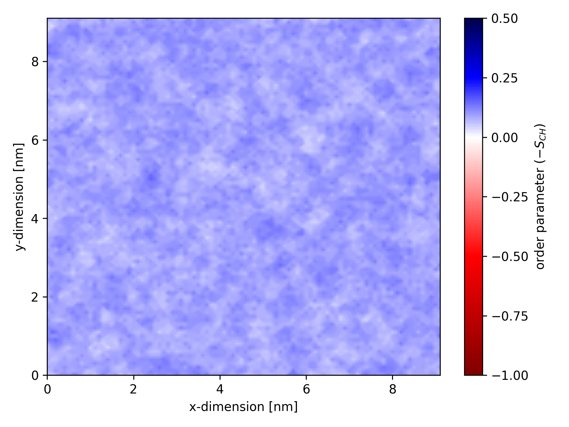
Ordermaps are especially useful for analyzing simulations involving transmembrane proteins. For such analyses, ensure the protein is centered and, ideally, RMSD-fitted in the trajectory.

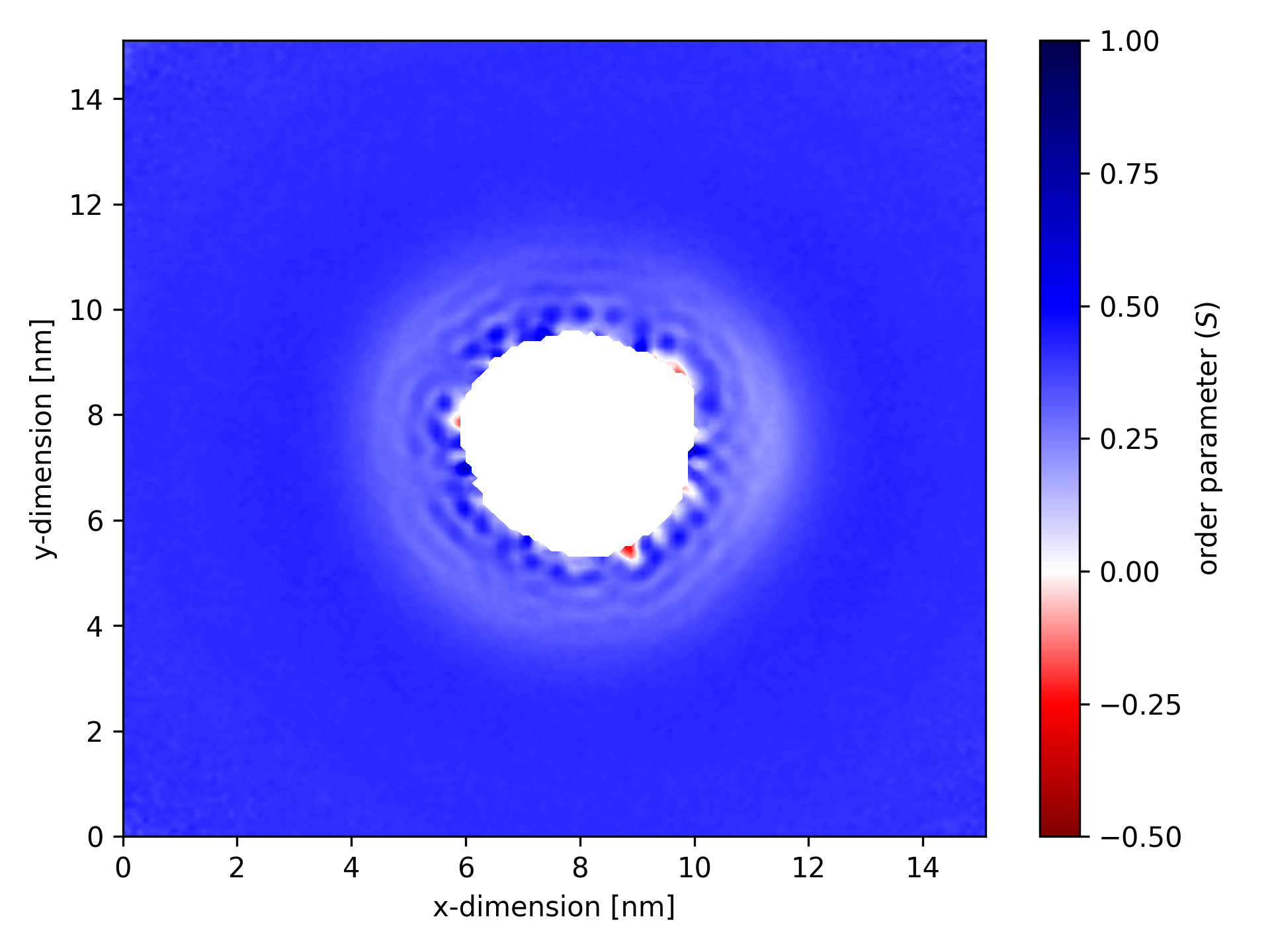
In this map of coarse-grained order for a particular lipid bond, the bright white region in the center represents the area occupied by the transmembrane protein. In this zone, no lipids (or an insufficient number to meet the min_samples threshold of 50) were detected. The membrane is disrupted in the vicinity of the protein.

Estimating errors

gorder is able to provide estimates of error for the individual bonds, atoms, and entire molecules.

The primary source of error when calculating order parameters from molecular dynamics simulations is the lack of convergence in the simulation. It’s also important to note that an order parameter calculated from a single trajectory frame is very unreliable unless the system is gigantic and contains many molecules. Using the standard deviation or standard error calculated from order parameters of individual frames or even samples is therefore not a viable option. Instead, gorder uses block averaging to calculate an error that reflects how well the simulation has converged.

To estimate the error, the trajectory is divided into blocks (default: 5). Each block represents a sequential portion of the trajectory: for example, the first fifth of the frames make up block #1, the second fifth forms block #2, and so on. The average order for each bond is calculated within each block, and a sample standard deviation is calculated from these block averages. This standard deviation is reported as the error. For simulations that are well-converged and have large enough blocks, the standard deviation between the blocks will be small.

Requesting error estimation

By default, gorder does not calculate error estimates. To enable error estimation, include the following line in your input YAML file:

estimate_error: true

The output YAML file will then include error estimates and may look similar to this:

# Order parameters calculated with 'gorder v0.5.0' using structure file 'system.tpr' and trajectory file 'md.xtc'.
average order:
  total:
    mean: 0.1631
    error: 0.0014
POPE:
  average order:
    total:
      mean: 0.1601
      error: 0.0015
  order parameters:
    POPE C22 (23):
      total:
        mean: 0.1036
        error: 0.0017
      bonds:
        POPE H2R (24):
          total:
            mean: 0.0876
            error: 0.0054
        POPE H2S (25):
          total:
            mean: 0.1196
            error: 0.0033
    POPE C32 (32):
      total:
        mean: 0.2297
        error: 0.0045
      bonds:
        POPE H2X (33):
          total:
            mean: 0.2423
            error: 0.0052
        POPE H2Y (34):
          total:
            mean: 0.2171
            error: 0.0045
#(...)

The errors are also reported in CSV and table files but not in XVG files:

molecule,residue,atom,relative index,total,total error,hydrogen #1,hydrogen #1 error,hydrogen #2,hydrogen #2 error,hydrogen #3,hydrogen #3 error
POPE,POPE,C22,23,0.1036,0.0017,0.0876,0.0054,0.1196,0.0033,,
POPE,POPE,C32,32,0.2297,0.0045,0.2423,0.0052,0.2171,0.0045,,
POPE,POPE,C23,35,0.2138,0.0034,0.2139,0.0025,0.2138,0.0047,,
POPE,POPE,C24,38,0.2165,0.0022,0.2158,0.0035,0.2172,0.0038,,
(...)

Molecule type POPE
                TOTAL       |    HYDROGEN #1    |    HYDROGEN #2    |    HYDROGEN #3    |
C22        0.1036 ± 0.0017  |  0.0876 ± 0.0054  |  0.1196 ± 0.0033  |                   |
C32        0.2297 ± 0.0045  |  0.2423 ± 0.0052  |  0.2171 ± 0.0045  |                   |
C23        0.2138 ± 0.0034  |  0.2139 ± 0.0025  |  0.2138 ± 0.0047  |                   |
C24        0.2165 ± 0.0022  |  0.2158 ± 0.0035  |  0.2172 ± 0.0038  |                   |
(...)

Error estimates are currently not available for individual ordermaps.

Changing the number of blocks

If you are unsatisfied with the default number of blocks (5), you can adjust this parameter:

estimate_error:
  n_blocks: 10

For example, setting n_blocks: 10 will use 10 blocks for error estimation instead of the default 5. You should avoid tweaking this number to get a lower error estimate.

Convergence analysis

gorder offers an additional method to assess simulation convergence by visualizing how the average order parameters evolve over time for individual molecules.

To request convergence analysis, include the following lines in your input YAML file:

estimate_error:
  output_convergence: convergence.xvg

This will not only estimate errors as described above but also generate an XVG file (e.g., convergence.xvg) which shows the order parameters calculated for each frame as the average of values from that frame and all preceding frames (i.e., prefix averages).

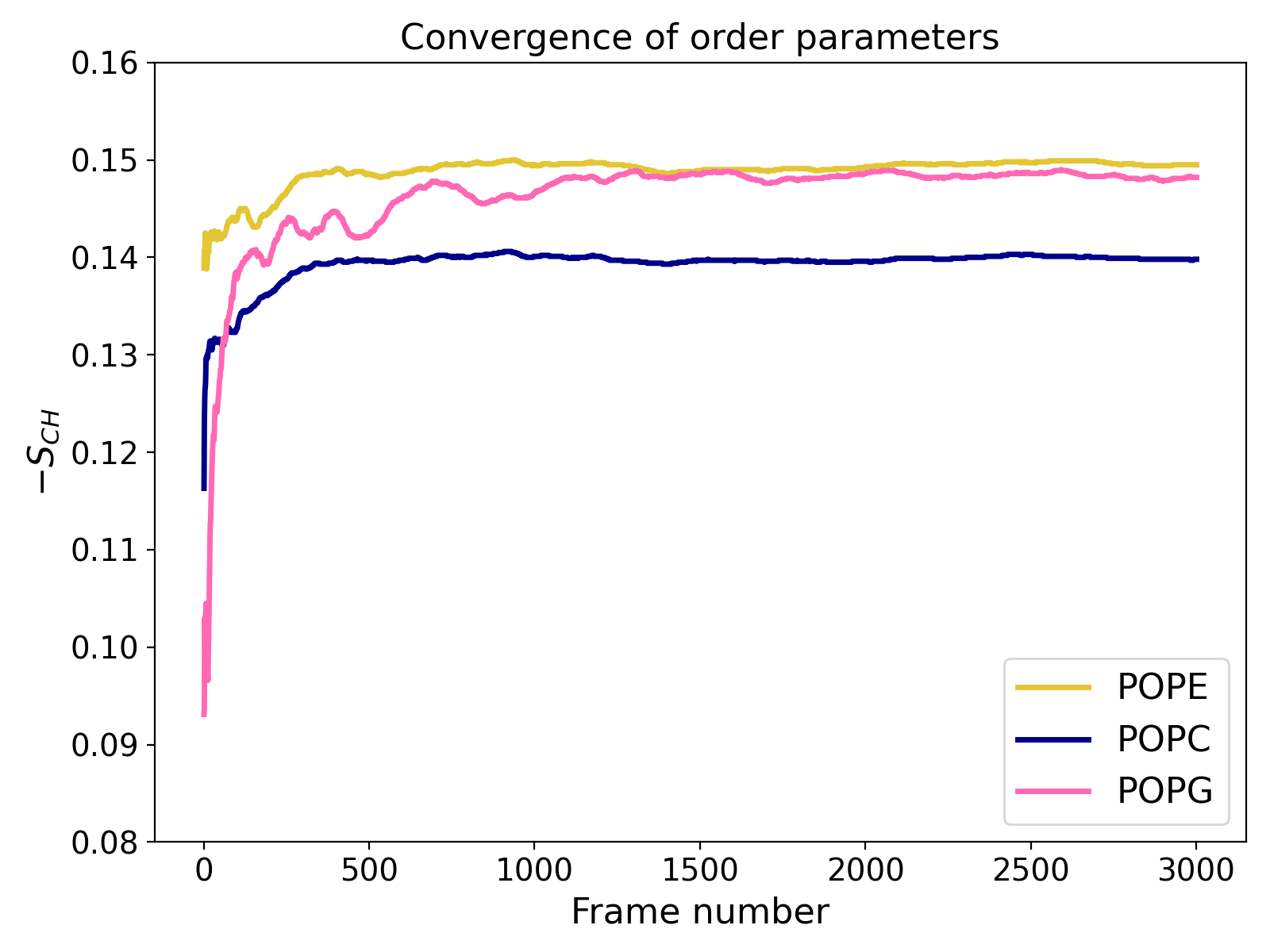
The example plot illustrates a relatively well-converged atomistic simulation where approximately 3,000 trajectory frames were analyzed. The chart shows that results for POPE and POPC lipids stabilize early (within the first third of the trajectory), while POPG converges more slowly (which is due to the smaller number of these lipids in the system).

Order parameters for a specific membrane region

gorder allows you to calculate order parameters for a specific region of the membrane within a defined geometric shape. Currently, three geometric shapes are supported for this selection: cuboid, cylinder, and sphere. When a geometric shape is specified, only bonds located within that shape are included in the order parameter calculations. The bond's inclusion is dynamically evaluated for every frame of the trajectory. This feature is useful for instance when analyzing order parameters near transmembrane proteins or specific membrane regions.

Note: The position of a bond is defined as the center of geometry of the bonded atoms.

Cuboidal selection

You can define a cuboid with specific dimensions and position to calculate order parameters for bonds within that region. To define a cuboid, include a configuration like the following in your input YAML file:

geometry: !Cuboid
  x: [2.0, 4.0]
  y: [1.0, 5.0]
  z: [0.0, 3.0]

This configuration calculates order parameters for bonds where the x-coordinate is between 2 and 4 nm, the y-coordinate is between 1 and 5 nm, and the z-coordinate is between 0 and 3 nm.

If a dimension is not specified, the cuboid is considered unbounded in that dimension, allowing bonds at any coordinate along that axis:

geometry: !Cuboid
  x: [2.0, 4.0]
  y: [1.0, 5.0]
  # the cuboid is infinite along the z-dimension

You can also define a reference point to make the cuboid dimensions relative instead of absolute:

geometry: !Cuboid
  reference: [3.0, 1.0, 0.0]
  x: [-2.0, 2.0]
  y: [1.0, 5.0]

In this example, the cuboid extends from 1 to 5 nm along the x-dimension, from 2 to 6 nm along the y-dimension, and remains infinite along the z-dimension. Periodic boundary conditions are also taken into account when constructing the cuboid.

The reference point can be defined as a static coordinate, a dynamic center of geometry of a specified group of atoms, or the center of the simulation box. For details, see Specifying the reference point.

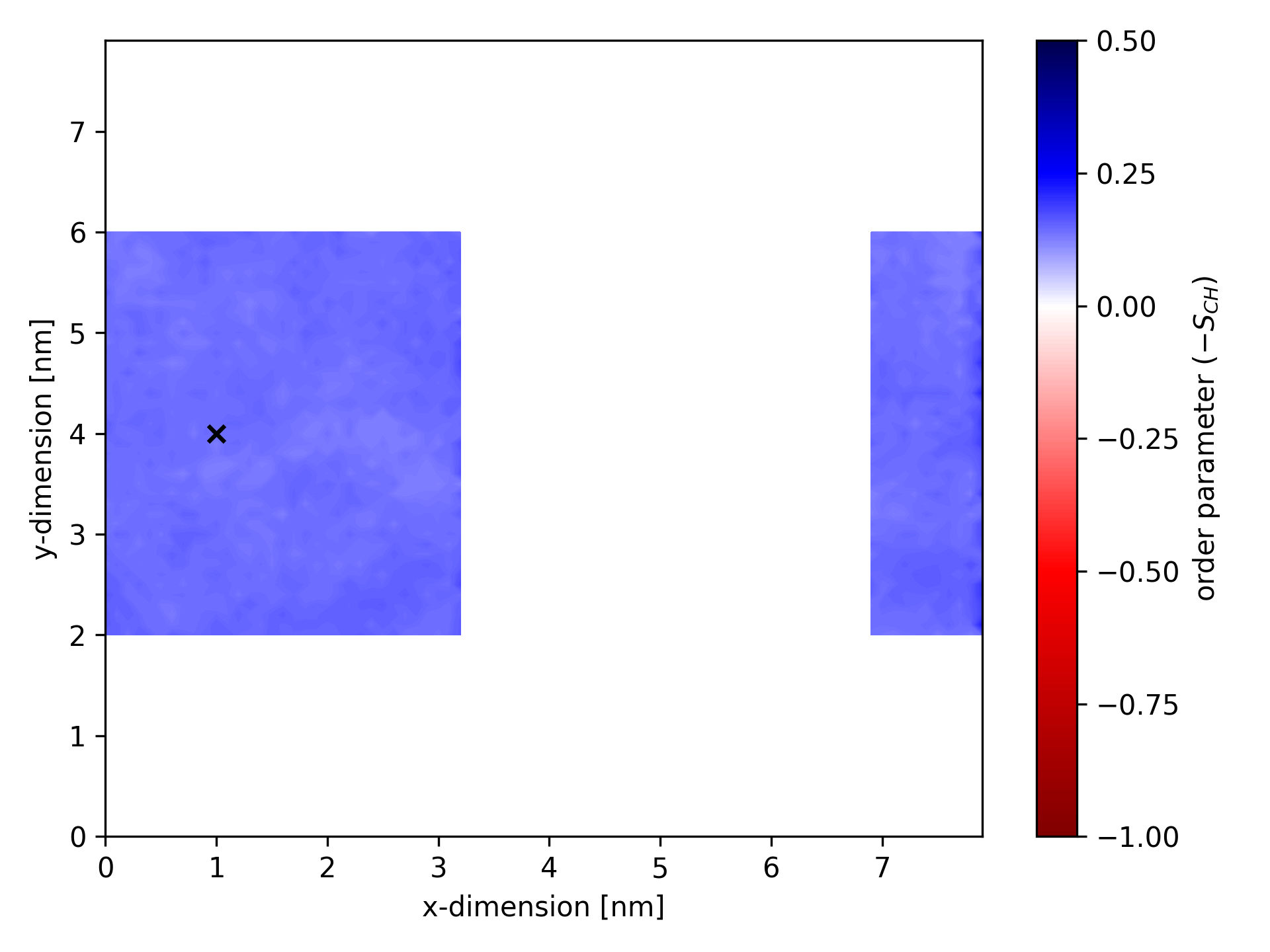
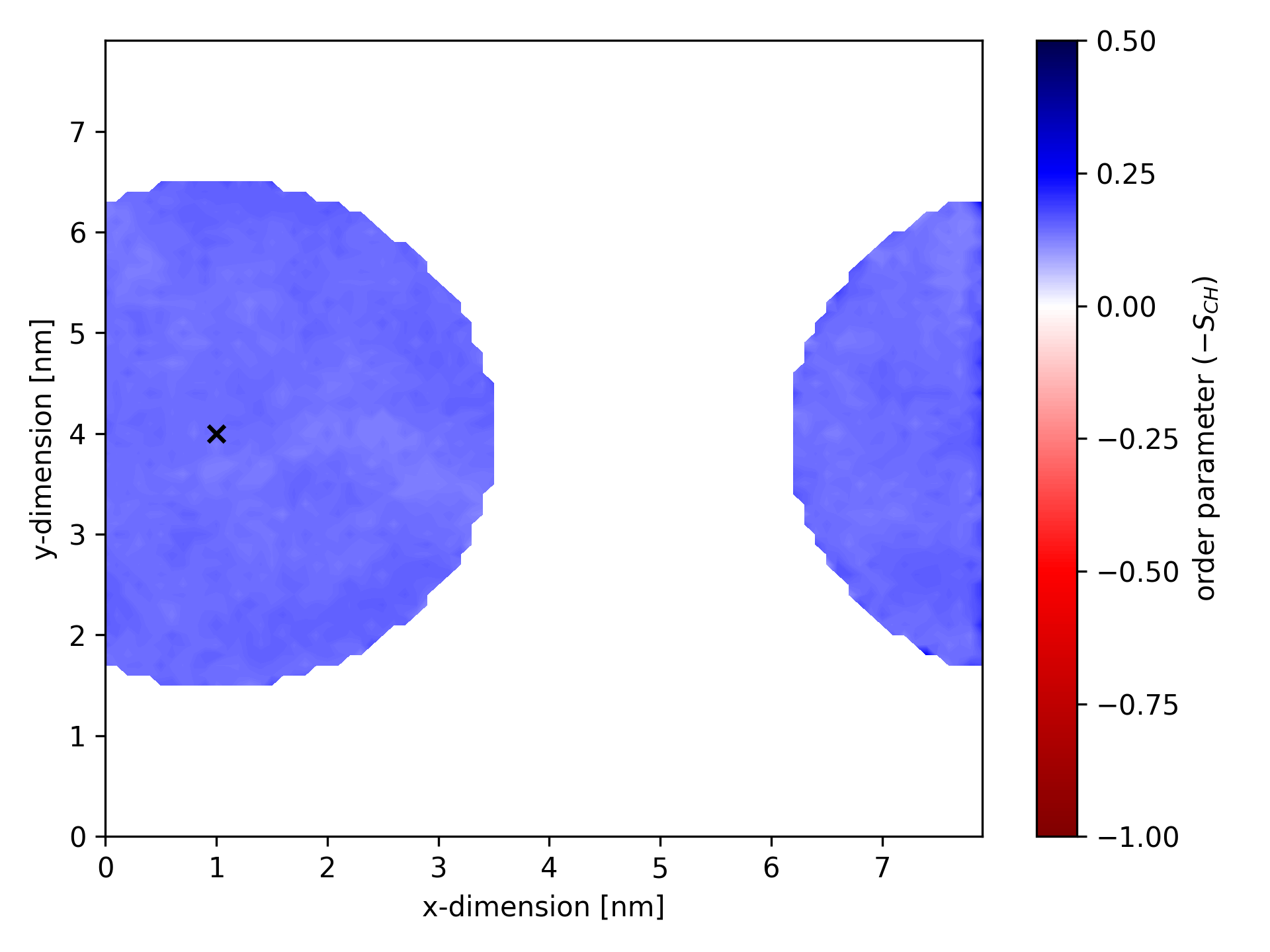
Below is an example of an ordermap where calculations considered only bonds within a specific cuboid. The static center of the cuboid is marked by a black ×.

Cylindrical selection

You can define a cylinder with specific dimensions, orientation, and position to calculate order parameters for bonds within that region. To specify a cylinder, include a configuration like the following in your input YAML file:

geometry: !Cylinder
  reference: [3.0, 1.0, 4.0]
  radius: 2.5
  span: [-1.0, 1.0]
  orientation: z

This configuration calculates order parameters for bonds within a cylinder centered at x = 3 nm, y = 1 nm, z = 4 nm. The cylinder is oriented along the z-axis, has a radius of 2.5 nm, and a height of 2 nm (spanning from z = 3 nm to z = 5 nm). Periodic boundary conditions are also taken into account when constructing the cylinder.

The reference point for the cylinder can be defined as a static coordinate, a dynamic center of geometry of a specified group of atoms, or the center of the simulation box. If the reference value is omitted, the origin of the simulation box [0, 0, 0] is used. For more details, see Specifying the reference point.

If the span parameter is omitted, the cylinder is considered infinitely long along its main axis (orientation):

geometry: !Cylinder
  radius: 2.5
  orientation: z

In this case, the cylinder is centered at the origin [0, 0, 0], has a radius of 2.5 nm, is oriented along the z-axis, and has an infinite height.

The main axis of the cylinder (orientation) must align with one of the simulation box dimensions. Only x, y, and z orientations are supported.

Below is an example of an ordermap where calculations considered only bonds within a specific cylinder (oriented along the membrane normal). The static center of the cylinder is marked by a black ×.

Spherical selection

You can define a sphere with a specific center and radius to calculate order parameters for bonds within that region. To specify a sphere, include a configuration like the following in your input YAML file:

geometry: !Sphere
  reference: [3.0, 1.0, 4.0]    # you can also use `center`
  radius: 2.5

This configuration calculates order parameters for bonds within a sphere centered at x = 3 nm, y = 1 nm, z = 4 nm, with a radius of 2.5 nm. Periodic boundary conditions are also considered when constructing the sphere.

The reference point (or center) for the sphere can be defined as a static coordinate, a dynamic center of geometry of a specified group of atoms, or the center of the simulation box. If the reference value is omitted, the sphere is centered at the origin of the simulation box [0, 0, 0]. For additional details, see Specifying the reference point.

Specifying the reference point

The reference point can be specified in one of three ways:

Static coordinates

Define a fixed reference point using explicit coordinates:

reference: [2.0, 2.5, 1.5]

This places the reference point at x = 2.0 nm, y = 2.5 nm, and z = 1.5 nm. Note that these coordinates are not scaled by the simulation box dimensions.

Dynamic center of geometry of selected atoms

Set the reference point as the center of geometry of a specified group of atoms:

reference: "@protein"

Here, the reference point corresponds to the geometric center of the @protein atom selection (all protein atoms in the system). The geometric center is recalculated for every frame of the trajectory. Use GSL syntax to specify the atom selection.

Dynamic simulation box center

Choose the center of the simulation box as the reference point:

reference: !Center

The reference point will be the geometric center of the simulation box in all three dimensions, recalculated for every frame of the trajectory.

If no reference point is specified, the default is the simulation box origin at [0, 0, 0].

Specifying membrane normal

gorder supports both static (provided by the user and applied to all lipid molecules throughout the entire analysis) and dynamic (calculated for each lipid molecule in each trajectory frame based on the actual membrane shape) membrane normal specification.

For planar membranes, the default static membrane normal is usually sufficient. However, for vesicles, you should always use dynamic membrane normal calculation. Keep in mind that computing the membrane normal dynamically is computationally expensive.

Static membrane normal

By default, gorder assumes the membrane normal is oriented along the z-axis, meaning the membrane is built in the xy-plane. If your membrane is oriented differently, you can manually specify the membrane normal in the input YAML file:

membrane_normal: x

In this example, the membrane normal is oriented along the x-axis, which means that the membrane is built in the yz-plane.

Only the primary axes of an orthogonal simulation box (x, y, and z) are supported as static membrane normals.

Dynamic membrane normal

If your membrane is non-planar, or if you want to use the actual membrane normal instead of an idealized direction, you can enable dynamic membrane normal calculation. In this case, you must specify the selection of 'head identifier' atoms (similar to when assigning lipids to leaflets):

membrane_normal: !Dynamic
  heads: "name P"

These 'head identifiers' are used to estimate the membrane surface and calculate the membrane normal for each lipid molecule. For consistency with leaflet classification, each analyzed lipid molecule must have exactly one head identifier; otherwise, an error will be raised.

The membrane normal is estimated for each lipid molecule in every frame. This is done by collecting the positions of 'head identifiers' located within a sphere around the molecule’s own head identifier and performing principal component analysis (PCA) on these positions. The last principal component (the direction with the least variation in atom positions) is then used as the membrane normal.

By default, the radius of the 'scanning sphere' is 2 nm, but you can adjust it in the input file:

membrane_normal: !Dynamic
  heads: "name P"
  radius: 1.5

The 'scanning sphere' must meet several requirements:

It must be large enough to include a sufficient number of lipid heads for reasonable principal component analysis.
It must be small enough to capture local membrane curvature correctly.
Most importantly, it must be small enough to avoid including head identifiers from the opposite membrane leaflet, as this would distort the calculated membrane normal.

As a general rule of thumb, set the radius to approximately half of the membrane thickness.

Limitations

When using dynamic membrane normal calculation, you should be aware of some limitations:

Ignoring periodic boundary conditions
When ignoring periodic boundary conditions, membrane normals for lipids located near the edges (and especially at the corners) of the simulation box might not be calculated accurately. This occurs because, without PBC, not all nearby lipid heads are included in the surface estimation. If periodic boundary conditions are considered (which is the default), this issue does not occur.
Assigning lipids to leaflets
All methods for classifying lipids into leaflets use the membrane normal to determine what is 'up' and what is 'down' in the membrane. However, due to technical limitations, these methods cannot use dynamically calculated membrane normals and always require a static membrane normal. You can specify this manually, for example:
```
leaflets: !Global
  membrane: "@membrane" 
  heads: "name P"
  membrane_normal: z
```
This membrane normal definition is used only when assigning lipids into leaflets. If you are working with a (reasonably) planar membrane, the membrane normal for leaflet classification does not need to be precise, so this approach is perfectly fine, even if you are otherwise working with dynamically calculated membrane normals. However, for a curved membrane, such as a vesicle, you should assign lipids into leaflets manually instead.
Constructing ordermaps
When constructing ordermaps, the plane in which an ordermap is generated is determined by the provided membrane normal. Since ordermaps can only be constructed in the xy, xz, or yz plane, they also require a static membrane normal (z, y, or x). If you are calculating the membrane normal dynamically and also want to construct ordermaps, you must specify the ordermap plane manually:
```
ordermaps:
  output_directory: "ordermaps"
  plane: xy
```

Analyzing a part of the trajectory

By default, gorder analyzes the entire provided trajectory, meaning it processes all frames from the start to the end of the trajectory.

If you want to analyze only a specific part of the trajectory, you can use the begin, end, and step options to control the time range and frequency of analysis.

begin: Specifies the time (in ps) from which the trajectory will start being read.
end: Specifies the time (in ps) at which the trajectory analysis will stop.
step: Specifies the step size for reading trajectory frames (i.e., how often a frame will be analyzed).

Example: Calculating coarse-grained order parameters from a specific part of a trajectory

structure: system.tpr
trajectory: md.xtc
analysis_type: !CGOrder
  beads: "@membrane"
begin: 100000.0
end: 300000.0
step: 5
output: order.yaml

In this example, the analysis starts at time 100,000 ps (100 ns) and ends at time 300,000 ps (300 ns). Every 5th frame of the trajectory will be analyzed.

Multithreaded analysis

The trajectory analysis can be performed using multiple threads. Utilizing more threads is generally much faster than using just one, although the speed gain also depends on the read performance of your storage device.

By default, gorder uses only 1 thread to perform the analysis. If you want to speed up the process by using multiple threads, you can specify the number of threads in your input YAML file:

n_threads: 4

In the example above, the analysis will be performed using 4 threads.

gorder guarantees binary identical output, regardless of the number of threads used.

Other options

Min samples

By default, gorder calculates order parameters for all bonds for which it collects at least one sample. If you want to increase the number of required samples, you can specify the minimum number of samples manually in the input YAML file:

min_samples: 10000

In this example, at least 10,000 samples are required for the bond to have a valid order parameter. If the number of samples is lower than this value, the order parameter will be NaN.

Overwrite

By default, gorder does not overwrite output files. Before writing an output file (or creating an output directory for the ordermaps), any existing file (or directory) with the same name is backed up. You can change this behavior by specifying the overwrite option in the input YAML file:

overwrite: true

In this example, no backups will be created, and files will be overwritten directly.

You can also specify this option on the command line when calling gorder:

$ gorder INPUT_YAML --overwrite

Silent

By default, gorder writes a lot of information about the progress of the analysis to the terminal (standard output). If you prefer not to see any of this information, you can specify it in the input YAML file:

silent: true

In this example, gorder will not write anything to standard output. Output files will still be generated, and the analysis will proceed as normal. If an error occurs, information about the error will be written to standard error output.

You can also specify this option on the command line when calling gorder:

$ gorder INPUT_YAML --silent

Manual lipid assignment to leaflets

If you do not want to use the automatic leaflet classification (described in Order parameters for individual leaflets), whether due to your system's complicated geometry or a lack of trust in the gorder assignment, you can manually specify the leaflet occupied by each lipid molecule (for each analyzed frame).

There are two ways to manually assign lipids to membrane leaflets: using NDX files or a "leaflet assignment file".

Assigning lipids using NDX file(s)

Using NDX files for lipid assignment is arguably a simpler method that enables seamless integration of gorder with FATSLiM, which implements possibly the best lipid classification method available.

NDX file

To begin, create an NDX file containing at least two groups. One group should contain lipid atoms (preferably just their 'head identifiers') of the upper leaflet, while the other group should contain lipid atoms of the lower leaflet.

[ UpperLeaflet ]
1140 1274 1810 2078 2212 2480 2614 2748 2882 3150 3284 3418 3686 3954 4088
4356 4490 4758 5026 5294 5428 5964 6098 6232 6366 6634 6902 7438 7572 7706
7974 8376 8778 8912 9046 9180 9582 9716 9850 10118 10386 10520 10654 10788 11056
11458 11592 11726 11860 12128 12262 12530 12664 13066 13200 13334 13602 14004 14272 14540
14808 14942 15076 15344 15478 15612 16014 16416 16818 17086 17354 17488 17622 17756 17890
18024 18158 18426 18694 18828 18962 19498 20034 20436 21106 21240 21508 21642 21776 21910
[ LowerLeaflet ]
1006 1408 1542 1676 1944 2346 3016 3552 3820 4222 4624 4892 5160 5562 5696
5830 6500 6768 7036 7170 7304 7840 8108 8242 8510 8644 9314 9448 9984 10252
10922 11190 11324 11994 12396 12798 12932 13468 13736 13870 14138 14406 14674 15210 15746
15880 16148 16282 16550 16684 16952 17220 18292 18560 19096 19230 19364 19632 19766 19900
20168 20302 20570 20704 20838 20972 21374 22044 22178 22312 22580 23116 23384 23518 23652

Using the NDX file

Then, specify the classification method in your configuration file:

leaflets: !FromNdx
  ndx: "leaflets.ndx"
  heads: "name P"
  upper_leaflet: "UpperLeaflet"
  lower_leaflet: "LowerLeaflet"
  frequency: !Once

The leaflet assignment will be read from the NDX file leaflets.ndx, which should contain two groups: UpperLeaflet and LowerLeaflet. These groups should include the atoms of the upper and lower leaflets, respectively. The heads field specifies the head identifiers for all analyzed lipid molecules. Note that each lipid molecule must have only one head identifier; otherwise, an error will be returned. Since we are using a single NDX file, we also need to specify frequency: !Once, ensuring that the leaflet assignment from the NDX file is applied to all analyzed trajectory frames.

The UpperLeaflet and LowerLeaflet groups may contain various atoms, but they must include all heads atoms for the lipids being analyzed. In other words, every analyzed lipid must be assigned to a leaflet. The NDX file itself can contain any number of additional groups, but for performance reasons, it is recommended to keep both the file and the specified groups as small as possible.

Scrambling-safe leaflet assignment

Instead of using a single NDX file, you can provide multiple NDX files, such as one file per trajectory frame. Your configuration file may then look like this:

leaflets: !FromNdx
#          first frame         second frame        third frame         fourth frame
  ndx: ["leaflets0001.ndx", "leaflets0002.ndx", "leaflets0003.ndx", "leaflets0004.ndx", (...)]
  heads: "name P"
  upper_leaflet: "UpperLeaflet"
  lower_leaflet: "LowerLeaflet"

With this setup, leaflet assignment will be performed for each frame using a different NDX file.

Specifying NDX files using `glob` pattern

Instead of manually listing many NDX file paths in the configuration file, you can use glob pattern matching:

leaflets: !FromNdx
  ndx: "leaflets*.ndx"
  heads: "name P"
  upper_leaflet: "UpperLeaflet"
  lower_leaflet: "LowerLeaflet"

This pattern matches all NDX files in the current directory whose names start with "leaflets", such as leaflets0001.ndx, leaflets0002.ndx, as well as leafletsABCD.ndx, leafletsX.ndx, and similar files, if they exist.

Glob returns files in lexicographic order based on filenames. As a result, leaflets10.ndx may appear before leaflets2.ndx. Always verify the order of NDX files and ensure that filenames are structured so that lexicographic and numerical ordering align. For example, when dealing with frames 1–9999, use filenames like leaflets0001.ndx to leaflets9999.ndx to maintain the correct order.

Assignments for every Nth frame

If you want to specify leaflet assignments for every Nth analyzed frame (e.g., every 10th frame), follow these steps:

Set the appropriate frequency in the configuration file. For example:

leaflets: !FromNdx
  ndx: ["leaflets0001.ndx", "leaflets0002.ndx", "leaflets0003.ndx", "leaflets0004.ndx", (...)]
  heads: "name P"
  upper_leaflet: "UpperLeaflet"
  lower_leaflet: "LowerLeaflet"
  frequency: !Every 10

Ensure that the number of provided NDX files exactly matches the number of analyzed frames divided by N. For example, if the trajectory is 10,000 frames long, every 5th frame is analyzed, and leaflet assignment is performed for every 10th analyzed frame, you must provide 200 NDX files. If you provide less or more NDX files, you will get an error during the analysis.

Assigning lipids using a leaflet assignment file

Another method for manually assigning lipids is using a YAML-formatted "leaflet assignment file". Unlike the NDX file method, where groups of atoms are used for assignment, the leaflet classification in this method is provided at the molecular level, with each molecule type having its own section in the file.

Leaflet assignment file

Consider a very small system consisting of 12 POPE molecules, 10 POPC molecules, and 8 POPG molecules. Let's say that this membrane is asymmetric:

The upper leaflet contains 12 POPE molecules and 4 POPG molecules.
The lower leaflet contains 10 POPC molecules and 4 POPG molecules.

The leaflet assignment file for this system should look as follows:

POPE:
  - [Upper, Upper, Upper, Upper, Upper, Upper, Upper, Upper, Upper, Upper, Upper, Upper]
POPC:
  - [Lower, Lower, Lower, Lower, Lower, Lower, Lower, Lower, Lower, Lower]
POPG:
  - [Upper, Upper, Upper, Upper, Lower, Lower, Lower, Lower]

Each position in each list corresponds to the leaflet occupied by one lipid molecule of the specified type. The molecules are listed in the order in which their first atoms appear in the input structure file.

Note: You can substitute Upper and Lower with 1 and 0, respectively, for specifying the 'upper' and 'lower' leaflets.

Using the leaflet assignment file

Save the leaflet assignment file, for example, as assignment.yaml. To use this file with gorder, include it in the YAML configuration file as follows:

leaflets: !FromFile
  file: assignment.yaml
  frequency: !Once

Ensure the frequency is set to !Once, as this leaflet assignment file provides information for only a single frame.

Inline specification of leaflet assignment

You can also embed the leaflet assignment directly in the configuration file:

leaflets: !Inline
  assignment:
    POPE:
      - [Upper, Upper, Upper, Upper, Upper, Upper, Upper, Upper, Upper, Upper, Upper, Upper]
    POPC:
      - [Lower, Lower, Lower, Lower, Lower, Lower, Lower, Lower, Lower, Lower]
    POPG:
      - [Upper, Upper, Upper, Upper, Lower, Lower, Lower, Lower]
  frequency: !Once

Scrambling-safe leaflet assignment

If lipid flip-flop occurs in your system, you may want to specify the leaflet assignment for each analyzed frame. For example:

POPE:
  # first analyzed frame
  - [Upper, Upper, Upper, Upper, Upper, Upper, Upper, Upper, Upper, Upper, Upper, Upper]
  # second analyzed frame
  - [Upper, Upper, Lower, Upper, Upper, Upper, Upper, Upper, Upper, Upper, Upper, Upper]
  # third analyzed frame
  - [Upper, Upper, Lower, Upper, Upper, Upper, Upper, Lower, Upper, Upper, Upper, Upper]
  # (...)
POPC:
  - [Lower, Lower, Lower, Lower, Lower, Lower, Lower, Lower, Lower, Lower]
  - [Lower, Lower, Lower, Lower, Lower, Lower, Lower, Lower, Lower, Upper]
  - [Lower, Lower, Lower, Upper, Lower, Lower, Lower, Lower, Lower, Upper]
  # (...)
POPG:
  - [Upper, Upper, Upper, Upper, Lower, Lower, Lower, Lower]
  - [Upper, Upper, Upper, Upper, Lower, Lower, Lower, Lower]
  - [Upper, Upper, Lower, Upper, Upper, Lower, Lower, Lower]
  # (...)

To use this expanded file, specify it in the YAML configuration file:

leaflets: !FromFile
  file: assignment.yaml
  frequency: !Every 1

Alternatively, since frequency: !Every 1 is the default setting, you can simplify the configuration:

leaflets: !FromFile assignment.yaml

Assignments for every Nth frame

If you want to specify leaflet assignments for every Nth analyzed frame (e.g., every 10th frame), you must:

Set the appropriate frequency in the configuration file. For example:
```
leaflets: !FromFile
  file: assignment.yaml
  frequency: !Every 10
```
Ensure that the number of frames in the leaflet assignment file exactly matches the number of analyzed frames divided by N. For example, if the trajectory is 10,000 frames long, every 5th frame is analyzed, and leaflet assignment is performed for every 10th analyzed frame, the leaflet assignment file must contain information for 200 frames.

Note: gorder is very opinionated when validating the leaflet assignment file. The file must specify the exact same number of lipid molecules for each molecule type as are present in the analyzed molecular system. Additionally, it must contain exactly the number of frames required for the leaflet assignment for the specified trajectory at the specified classification frequency (i.e., not a single unused frame can be present in the leaflet assignment file). The leaflet assignment file also cannot include information about molecule types that do not exist in the system. If any of these criteria are not met, gorder will reject the leaflet assignment file. This strict validation reduces the chance of errors, as mistakes in manual assignments are easy to make but can be very difficult to detect otherwise.

Using other input file formats

gorder is primarily designed for analyzing Gromacs simulations. The most efficient and straightforward way to use it is therefore by providing it with a TPR file and an XTC file. However, to make it more flexible and less dependent on a specific MD engine, gorder also supports various other file formats for both structure/topology and trajectory files.

Structure and topology file formats

In rare cases where gorder cannot read your input TPR file, or if no TPR file is available, you can provide the system structure and topology using alternative file formats. gorder supports GRO, PDB, and PQR files as structure files.

For example, the following YAML input file is valid if the provided PDB file includes a connectivity section (and has fewer than 100,000 atoms due to PDB format limitations):

structure: system.pdb
trajectory: md.xtc
analysis_type: !CGOrder
  beads: "@membrane"
output: order.yaml

If the PDB file lacks a connectivity section or if you are using a GRO or PQR file as the input structure, you must also supply a "bonds" file:

structure: system.gro
bonds: system.bnd   # the file extension does not matter here
trajectory: md.xtc
analysis_type: !CGOrder
  beads: "@membrane"
output: order.yaml

Connectivity information will be read from system.bnd. Note that the connectivity data in the bonds file overrides even information in the provided PDB or TPR file.

gorder identifies the file format based on the file extension: .tpr for TPR files, .gro for GRO files, .pdb for PDB files, and .pqr for PQR files. Ensure that the file is named correspondingly.

Specification of the bonds file

The bonds file format is similar to the PDB connectivity block but simpler and much more flexible. It also supports systems of any (reasonable) size.

Each line in the file contains numbers separated by whitespace. The first number specifies the "target atom" (serial number), and the following numbers specify the atoms bonded to it. Serial numbers correspond to Gromacs numbering, where the first atom is 1, the second is 2, and so on (no matter the "atom number" in the input GRO or PDB file).

1 2 4

In this example, atom 1 is bonded to atoms 2 and 4. Atoms 2 and 4 are not bonded to each other.

Each bond needs to be specified only once (with any order of atoms), but duplicating entries is allowed. For instance, the following bonds files are equivalent:

1 2 4
2 3

(The system contains three bonds: atoms 1 and 2, atoms 1 and 4, and atoms 2 and 3.)

Bonds can be listed in any order, and multiple lines can start with the same target atom. Any number of bonds can be specified on one line. Empty lines are ignored, and any amount of whitespace is allowed between the numbers. Comments can be added using #:

1 2 4   # atom 1 is bonded to atoms 2 and 4
2 3

Here’s an excerpt from an example bonds file:

# Example bonds file for an atomistic system
1 2 3 4 5
2 1
3 1
4 1
5 1 6 7 8
6 5
7 5
8 5 9 10 15
9 8
10 8
11 12 13 14 15
12 11
13 11
14 11 16
15 8 11
16 14 17 18 19
# (...)

Note about selecting elements

When using the element keyword in GSL atom selection queries, atoms are selected based on their associated element. Element information is natively available in TPR files but is missing in other supported formats. If a non-TPR file is used, gorder will attempt to guess the elements of atoms based on the atom and residue names.

If gorder detects potential issues with the guess, it will display a warning in the terminal. You can then evaluate whether the concerns are harmless, avoid using the element keyword, or provide a TPR file instead.

Trajectory file formats

gorder is highly optimized to read XTC files as quickly as possible. If you have an XTC file or can generate one, it is recommended to use it. However, gorder also supports various other trajectory file formats, namely TRR, GRO, PDB, Amber NetCDF, DCD, and LAMMPSTRJ. You can use any of these files instead of an XTC trajectory, and gorder will automatically recognize the format based on the file extension.

gorder identifies the file format based on the file extension: .xtc for XTC files, .trr for TRR files, .gro for GRO files, .pdb for PDB files, .nc for Amber NetCDF files, .dcd for DCD files, and .lammpstrj for LAMMPSTRJ files. Ensure that your trajectory file is named accordingly.

Note that some features of gorder are not available for certain trajectory file formats. Specifically, do not specify the analysis time range using begin and end if your trajectory file is a PDB file or an Amber NetCDF file. This will not work and will result in an error!

You can only use this feature with a GRO trajectory if the file contains simulation time and step information in the 'title' line, formatted as follows:

Some Arbitrarily Long Title (...) t= SIMULATION_TIME step= SIMULATION_STEP

For example:

System t= 100.00000 step= 5000

Additionally, note that gorder assumes that time information in DCD files is specified in ps.

Ignoring periodic boundary conditions

gorder fully supports the handling of orthogonal (i.e., rectangular cuboid) periodic boundary conditions (PBC) applied in all three dimensions. If your simulation box is orthogonal and PBC are applied in all three dimensions, you can use a raw trajectory generated by Gromacs directly, without worrying about making molecules whole in the simulation box or dealing with other PBC-related issues. gorder will handle everything automatically.

However, if your simulation box is not orthogonal, gorder cannot properly treat the system and you will get an error. In such cases, you must instruct gorder to ignore periodic boundary conditions by adding the following line to your input YAML file:

handle_pbc: false

When this option is set to false, gorder will disregard periodic boundary conditions and the presence of any simulation box. Effectively, it will treat the atoms in your system as if they exist in an infinite, unbound environment. When ignoring PBC, it is crucial to ensure that all lipid molecules in your system are whole in every frame of the input trajectory. If your molecules are "broken" at the box boundaries, you may silently get completely incorrect results! When ignoring PBC, you will always get a warning reminding you to make molecules whole:

[W] Periodic boundary conditions ignored. Lipid molecules must be made whole!

With Gromacs, you can make molecules whole using the following command:

gmx trjconv -s TPR_FILE -f XTC_FILE -pbc mol -o OUTPUT_XTC_FILE

The resulting OUTPUT_XTC_FILE should then be used as the trajectory input for gorder.

You can of course choose to ignore PBC for any system, even if it has an orthogonal box.

Note: You do not necessarily have to set handle_pbc to false when working with an orthogonal box with PBC applied in fewer than three dimensions. However, such systems are untested, so proceed with caution. In case you are not sure the analysis is correct, try using a trajectory with whole molecules, set handle_pbc to false, and check whether the results change.

Limitations when ignoring PBC

Be aware of the following limitations when PBC are ignored:

Order parameters for individual leaflets
Ensure that your membrane is fully within the simulation box. For example, if your membrane lies in the xy-plane, ensure it does not extend beyond the limits of the simulation box in the z-dimension or appear fragmented across the periodic boundary. Failing to meet this requirement may result in entirely incorrect lipid leaflet assignments. To avoid issues, you may want to center the membrane in the simulation box before running the analysis.
Ordermap dimensions
When constructing ordermaps, you cannot automatically derive their dimensions from the simulation box because it is ignored. You must specify the dimensions manually. Forgetting to do this will result in an error. See this section of the manual for instructions on setting dimensions.
Reference points for geometry selections
When calculating order parameters for a specific region, you cannot use the dynamic center of the simulation box as the reference point because gorder ignores box information. If this constraint is violated, you will get an error. However, you can still use static coordinates or the dynamic center of geometry as the reference point. If using the dynamic center of geometry, ensure that your selected atoms for center calculation are made whole, i.e., are not broken at the simulation box boundary.
Using structures and trajectories not generated by Gromacs
While gorder (and Gromacs) interpret [0, 0, 0] as the origin of the simulation box (i.e., one of its corners), some other software treats [0, 0, 0] as the center of the simulation box. This difference can cause issues when ignoring periodic boundary conditions, as particles may not be correctly wrapped into the box as gorder expects. In such cases, you must translate the system by half of box size in each dimension so that [0, 0, 0] aligns with the origin of the simulation box (rather than its center) before running the analysis.

Extracting all analysis options

When gorder runs, it automatically sets many analysis options to their default values if they are not explicitly specified. To view the full set of parameters used in an analysis, including defaults, you can run the gorder program with the --export-config argument. For example:

$ gorder analyze.yaml --export-config analyze_out.yaml

The file analyze_out.yaml will contain all the input parameters for the analysis, including:

parameters specified in the input configuration file,
parameters provided on the command line, and
default values filled in by gorder.

This output file can also be used as a valid input configuration file for subsequent gorder runs.

Using `gorder` as a Rust crate

gorder can also be used as a Rust crate, allowing you to call it directly from your Rust code.

To use gorder in your project, first add it as a dependency:

$ cargo add gorder

Next, include the crate into your Rust code:

#![allow(unused)]
fn main() {
use gorder::prelude::*;
}

Once imported, you can access all the options and functionality described in this manual.

For instance, the following input YAML file:

structure: system.tpr
trajectory: md.xtc
analysis_type: !CGOrder
  beads: "@membrane"
output: order.yaml

can also by written as the following Rust code:

#![allow(unused)]
fn main() {
let analysis = Analysis::builder()
    .structure("system.tpr")
    .trajectory("md.xtc")
    .analysis_type(AnalysisType::cgorder("@membrane"))
    .output("order.yaml")
    .build()?;
}

You can then run the analysis like this:

#![allow(unused)]
fn main() {
let results = analysis.run()?;
}

and either write the results into the output file(s):

#![allow(unused)]
fn main() {
results.write()?;
}

or access them programmatically.

See the Rust API documentation on docs.rs for more information about using gorder as a Rust crate.

Limitations

While gorder aims to provide accurate and reliable results, there are some known limitations and scenarios where it may not be suitable. The current limitations are as follows:

gorder cannot read TPR files generated with Gromacs versions older than 5.1.
- Why is this the case? This limitation stems from the minitpr crate used to parse TPR files. The TPR file format evolves constantly, and supporting all ancient Gromacs versions is simply not feasible.
- What can you do if your TPR file is this old? In most cases, the solution is simple: generate a TPR file using a newer version of Gromacs. Since gorder only needs the system topology, you can use gmx grompp with any MDP file to create an updated TPR file. If generating a new TPR file is not an option for you, you can instead provide a PDB file with a connectivity section or a GRO file along with a bonds file (see Using other input file formats).
- Will this be addressed in the future? Older Gromacs versions will likely never be fully supported.
gorder only fully supports systems with orthogonal simulation boxes and periodic boundary conditions applied in all three dimensions.
- Why is this the case? This limitation arises from the groan_rs crate, which provides only partial support for non-orthogonal simulation boxes. Handling periodic boundary conditions in such boxes is complex and not fully implemented at present.
- What can you do if your box is not orthogonal? You must instruct gorder to ignore periodic boundary conditions. Then, provide a trajectory where the lipid molecules are whole, and perform the analysis as usual.
- What can you do if your system is not periodic in some dimensions? In most cases, there will be no issue; however, such systems have not been tested, and artifacts may occur. You can try ignoring periodic boundary conditions while ensuring the lipid molecules are whole and verify if the results change.
- Will this be addressed in the future? gorder is unlikely to ever fully support non-orthogonal simulation boxes, simply because they are not common in membrane simulations. However, better support for partially periodic systems might be added in the future.
gorder does not fully support the analysis of systems with multiple membranes.
- Why is this the case? Handling multiple membranes is complex, and such systems are relatively uncommon. gorder is primarily designed for analyzing single-membrane systems. This does not mean you cannot use it for multi-membrane systems, but some features may not work as expected (see below).
- What can you do if your system contains multiple membranes? If you are performing basic analysis with a static membrane normal and no leaflet assignment, no special action is required. However, be aware that order parameters from all membranes will be averaged into a single collective set of order parameters. If you are assigning leaflets, note that the only usable classification method is the individual method (assuming the membranes are planar, since for vesicles, you should always assign lipids to leaflets manually). If you are using dynamic membrane normal calculation, ensure that the membranes are sufficiently far apart: specifically, farther than the radius value used in the membrane normal calculation. You can of course also select atoms from a single membrane for analysis, but make sure to consistently apply this selection across all relevant sections, particularly in dynamic membrane normal calculation.
- Will this be addressed in the future? Will gorder ever support membrane-specific order parameter calculations? This is highly unlikely. Multi-membrane systems are rare, and membrane-wise analysis can be approximated by running individual analyses with different atom selections. Since gorder is fast (and even faster when the trajectory is already cached), performing multiple runs should not be a significant issue.

Feedback

If you encounter an issue with the program, such as incorrect or unexpected behavior or functionality, please open an issue on GitHub or send an email to ladmeb@gmail.com.

For feature requests, concerns about calculation methods or metrics, or improvement suggestions, please use the same contact methods. If you discover software you believe outperforms gorder in lipid order calculations or simply does something better, sharing your feedback is encouraged. Any constructive criticism, even negative, is welcome.

If you enjoy using gorder, you can show your support by starring ★ the project on GitHub or recommending it to others.

Citing

If you would like to cite the gorder software, use the following BibTeX entry:

@software{gorder,
  author       = {Ladislav Bartos},
  title        = {gorder},
  month        = dec,
  year         = 2024,
  publisher    = {Zenodo},
  doi          = {10.5281/zenodo.14391305},
  url          = {https://doi.org/10.5281/zenodo.14391305}}

gorder manual